After having used the tidyverse toolkit for a while to wrangle data in R, i recently switched to the data.table package. I found this page very helpful to grasp the power of data.table.
For dataset bigger than 1GB than can fit into the RAM, read, write, filter and aggregations operations are 10 to 100 times faster than the dplyr/base R tools.
On top of that, i found its syntax extremely concise, like writing Haiku in R. I started learning R using the dplyr/tidyr packages three years ago, and switching to data.table is a logical evolution.
As a Zwift player, i explored their API with the help of data.table.
Zwift players overview
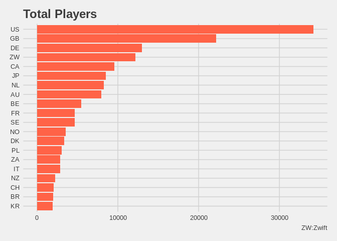
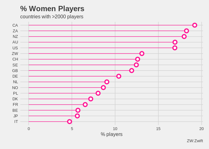
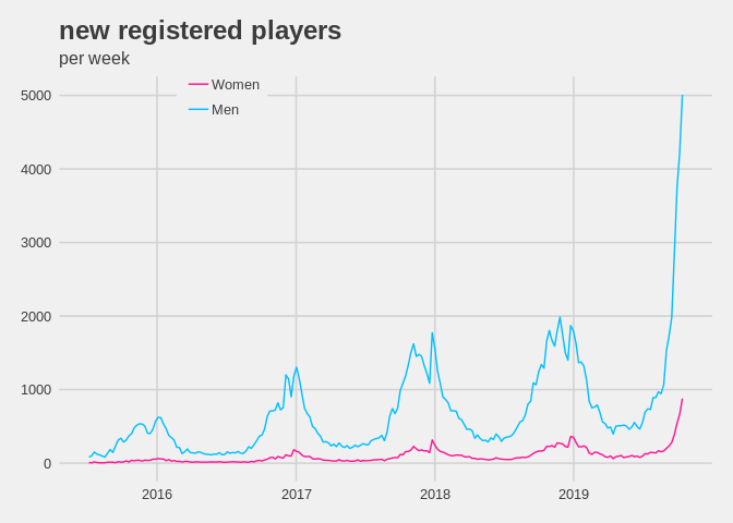
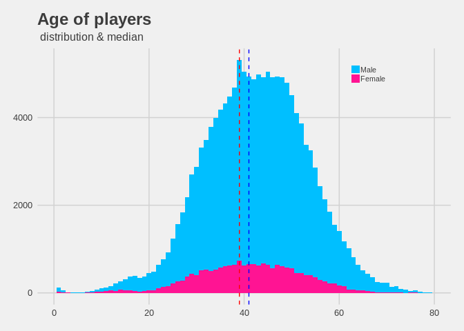
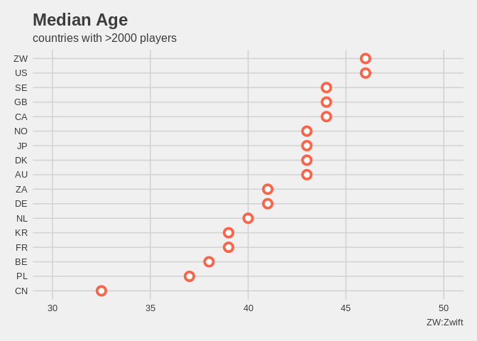
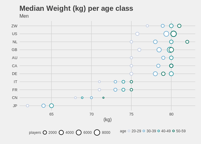
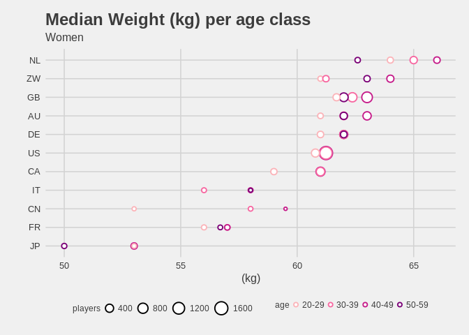
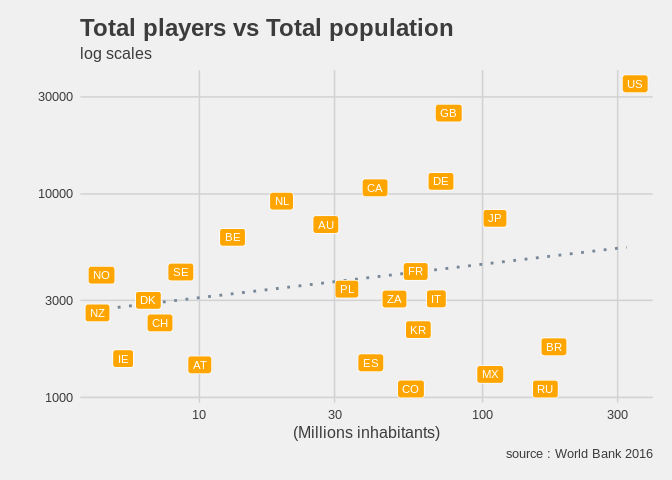
Using logged in players data scrapped from the Zwift API between 17th to 25th October, we can have a look at how does the Zwifter population looks like.
Final thought:
Using the activity data, i tried to figure out whether the evolution over the time of the average Watts (per ride duration) was somehow related to other features but could not come to any significant relationships.
- The source code is available here.
- i used the python Zwift client package to scrap the data.